Empirical dynamic modeling (EDM) is an emerging data-driven framework for modeling nonlinear dynamic systems. EDM is based on the mathematical theory of reconstructing system attractors from time series data (Takens 1981). Many scientific fields use models as approximations of reality in order to test hypothesized mechanisms, explain past observations and predict future outcomes. In most cases these models are based on hypothesized parametric equations or known physical laws that describe simple idealized situations such as controlled single-factor experiments, but do not apply to more complex natural settings. Empirical models, that infer patterns and associations from the data (instead of using hypothesized equations), represent an alternative and highly flexible approach.
The basic underlying goal of EDM is to reconstruct the behavior of dynamic systems from time series data. This approach is based on mathematical theory developed initially by (Takens 1981), and expanded on by others (Casdagli et al. 1991, Sauer et al. 1991, Deyle and Sugihara 2011). Because these methods operate with minimal assumptions, they are particularly suitable for studying systems that exhibit non-equilibrium dynamics and nonlinear state-dependent behavior (i.e. where interactions change over time and as a function of the system state).
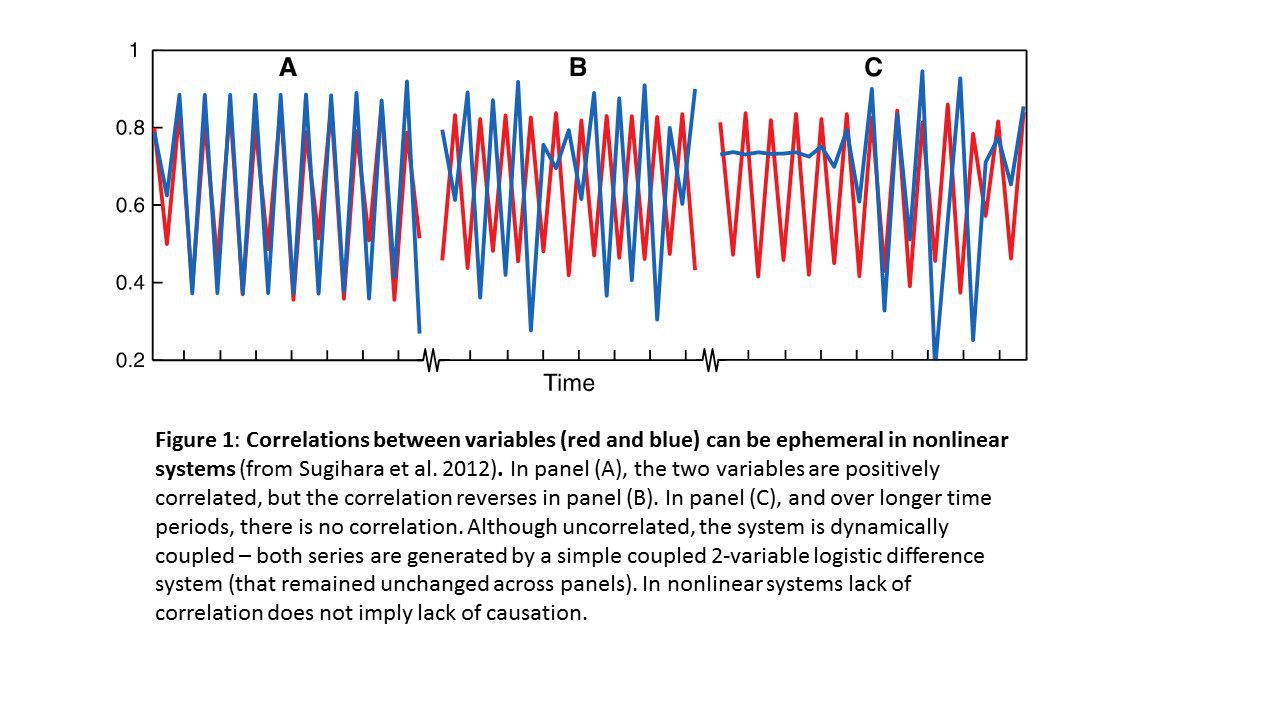
“Lack of correlation does not imply lack of causation.”
Current analytics in many scientific fields are rooted in a linear statistical paradigm inherited from engineering and rely on correlation-based inferences. But beyond the obvious fact that some correlations will be spurious, there may be many real interactions that are invisible when using correlation-based tests: two genes that interact in a nonlinear fashion can produce periods of positive, negative, or no correlation among their expression (the phenomenon of “mirage correlations”; Sugihara et al. 2012). Indeed, even simple nonlinear processes are known to give rise to the phenomenon of “mirage correlations” where variables can appear to be correlated, but this correlation may vanish or even change sign over different time periods (Figure 1). Such transient correlations can produce the appearance of non-stationarity that can obscure any statistical association, and more importantly they can suggest that coupled variables are not causally related at all. Thus, in a linear system, just as “correlation does not imply causation”, in a nonlinear system lack of correlation does not imply lack of causation. Therefore, for systems of nonlinear interacting parts, correlation, though insidiously ingrained in our thinking, is fundamentally the wrong tool for analysis.
The fact that nonlinear and dynamic behavior is ubiquitous in complex systems represents a mismatch for current linear methods (e.g. principal components, k-means clustering) that treat systems as essentially static. Ignoring the time domain by assuming constancy is an expedient that carries a high cost in a nonlinear (context-dependent) world. To illustrate this latter point, consider the following example involving time-course data on yeast gene expression obtained by the Verma Lab at The Salk Institute:
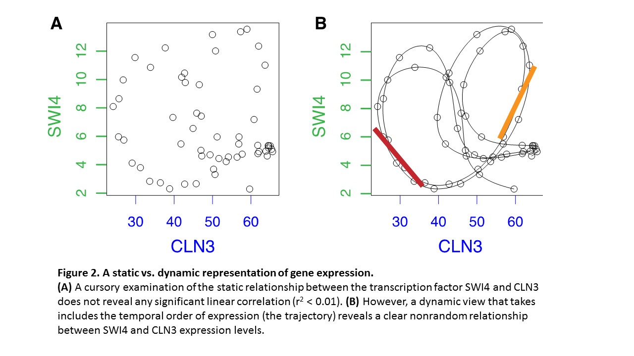
Note that the trajectories running through this cloud of points describes how the interrelationships vary through time. As the state of the cell changes according to the rules that describe the system of genes as they express (the internal cell dynamics), this traces out a trajectory. Taken together the trajectories form an attractor – a geometric object formed from the collection of trajectories (Figure 3). As a dynamical system, these trajectories and the resulting attractor display the changing relationship of coordinate variables to each other.
“Taken’s Idea”
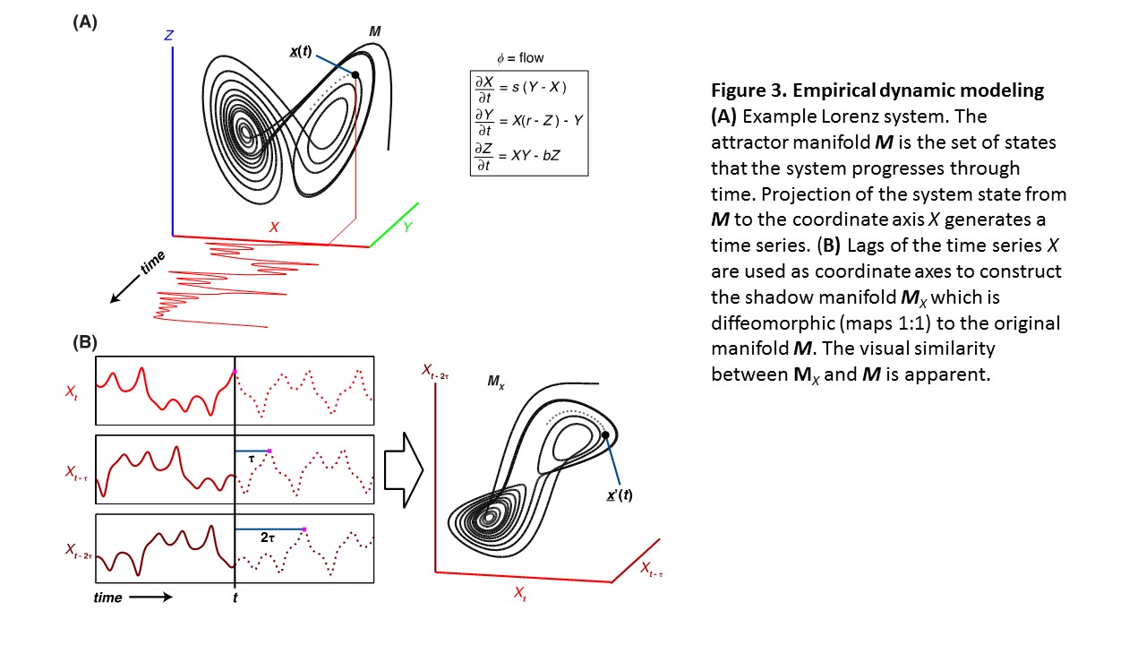
Briefly, in EDM the state of a dynamical system can be thought of as a location in a state space, whose coordinate axes are the relevant interacting variables (relevant interacting species of an ecosystem or genes of a cell etc). The system state changes and evolves in time according to the rules/equations that describe the system dynamics, and this traces out a trajectory. The collection of these time-series trajectories forms a geometric object known as an attractor manifold, which describes empirically how variables (e.g. genes and their expression levels) relate to each other in time—hence “empirical dynamic modeling” (EDM).
Conversely, each variable can be thought of as a projection of the system state onto a particular coordinate axis. In other words, a time series is simply the projection of the motion of the system onto a particular axis, and recorded over time. As such, each time series contains information about the underlying system dynamics (link to multiembed). In fact, Takens’ embedding theorem shows that each variable contains information about all the others, which quite remarkably allows systems to be studied from just a single time-series (Takens 1981) by taking time-lag coordinates of the single variable as proxies for the other variables (Figure 3).
For more information on EDM, please visit the Video Animations page under the Research tab.